 1
 2
 3
 4
 5
 6
 7
 8
 9
10
11
12
13
14
15
16
17
|
from __future__ import print_function

import matplotlib.pyplot as plt
import numpy as np
import pandas as pd
import torch
import torch.nn as nn
import torch.nn.functional as F
import torch.optim as optim
from linformer import Linformer
from sklearn.model_selection import train_test_split
from torch.optim.lr_scheduler import StepLR
from torch.utils.data import DataLoader, Dataset
from torchvision import datasets, transforms
from tqdm.notebook import tqdm
import torchvision
from vit_pytorch.efficient import ViT
|
1
2
3
4
5
6
7
8
|
print(f"Is CUDA supported by this system? {torch.cuda.is_available()}")
print(f"CUDA version: {torch.version.cuda}")

# Storing ID of current CUDA device
cuda_id = torch.cuda.current_device()
print(f"ID of current CUDA device: {torch.cuda.current_device()}")

print(f"Name of current CUDA device: {torch.cuda.get_device_name(cuda_id)}")
|
Is CUDA supported by this system? True
CUDA version: 11.7
ID of current CUDA device: 0
Name of current CUDA device: NVIDIA GeForce RTX 4090
Pre Processing
Load Data
Here we are loading the CIFAR100 data set using the built-in function from PyTorch.
1
2
3
4
5
6
7
8
|
batchSize = 128

# Orginial data is list of tuples (PIL Image, class label)
# train_split  = torchvision.datasets.CIFAR100('./cifar-100', train=True,download=True,  transform = transforms.Compose([transforms.ToTensor()]))
# test_split  = torchvision.datasets.CIFAR100('./cifar-100', train=False,download=True,  transform = transforms.Compose([transforms.ToTensor()]))

train_split  = torchvision.datasets.CIFAR100('./cifar-100', train=True,download=True)
test_split  = torchvision.datasets.CIFAR100('./cifar-100', train=False,download=True)
|
Files already downloaded and verified
Files already downloaded and verified
(<PIL.Image.Image image mode=RGB size=32x32>, 19)
Each element in the train and test split contains an image in tensor and its class label. Here’s a dictionary that translate the number class labels to text labels.
  1
  2
  3
  4
  5
  6
  7
  8
  9
 10
 11
 12
 13
 14
 15
 16
 17
 18
 19
 20
 21
 22
 23
 24
 25
 26
 27
 28
 29
 30
 31
 32
 33
 34
 35
 36
 37
 38
 39
 40
 41
 42
 43
 44
 45
 46
 47
 48
 49
 50
 51
 52
 53
 54
 55
 56
 57
 58
 59
 60
 61
 62
 63
 64
 65
 66
 67
 68
 69
 70
 71
 72
 73
 74
 75
 76
 77
 78
 79
 80
 81
 82
 83
 84
 85
 86
 87
 88
 89
 90
 91
 92
 93
 94
 95
 96
 97
 98
 99
100
101
102
|
textLabel = [
'apple', # id 0
'aquarium_fish',
'baby',
'bear',
'beaver',
'bed',
'bee',
'beetle',
'bicycle',
'bottle',
'bowl',
'boy',
'bridge',
'bus',
'butterfly',
'camel',
'can',
'castle',
'caterpillar',
'cattle',
'chair',
'chimpanzee',
'clock',
'cloud',
'cockroach',
'couch',
'crab',
'crocodile',
'cup',
'dinosaur',
'dolphin',
'elephant',
'flatfish',
'forest',
'fox',
'girl',
'hamster',
'house',
'kangaroo',
'computer_keyboard',
'lamp',
'lawn_mower',
'leopard',
'lion',
'lizard',
'lobster',
'man',
'maple_tree',
'motorcycle',
'mountain',
'mouse',
'mushroom',
'oak_tree',
'orange',
'orchid',
'otter',
'palm_tree',
'pear',
'pickup_truck',
'pine_tree',
'plain',
'plate',
'poppy',
'porcupine',
'possum',
'rabbit',
'raccoon',
'ray',
'road',
'rocket',
'rose',
'sea',
'seal',
'shark',
'shrew',
'skunk',
'skyscraper',
'snail',
'snake',
'spider',
'squirrel',
'streetcar',
'sunflower',
'sweet_pepper',
'table',
'tank',
'telephone',
'television',
'tiger',
'tractor',
'train',
'trout',
'tulip',
'turtle',
'wardrobe',
'whale',
'willow_tree',
'wolf',
'woman',
'worm',
]
|
Insepct Data
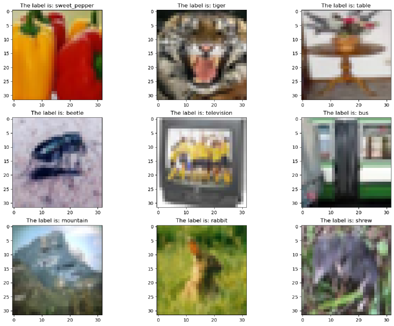
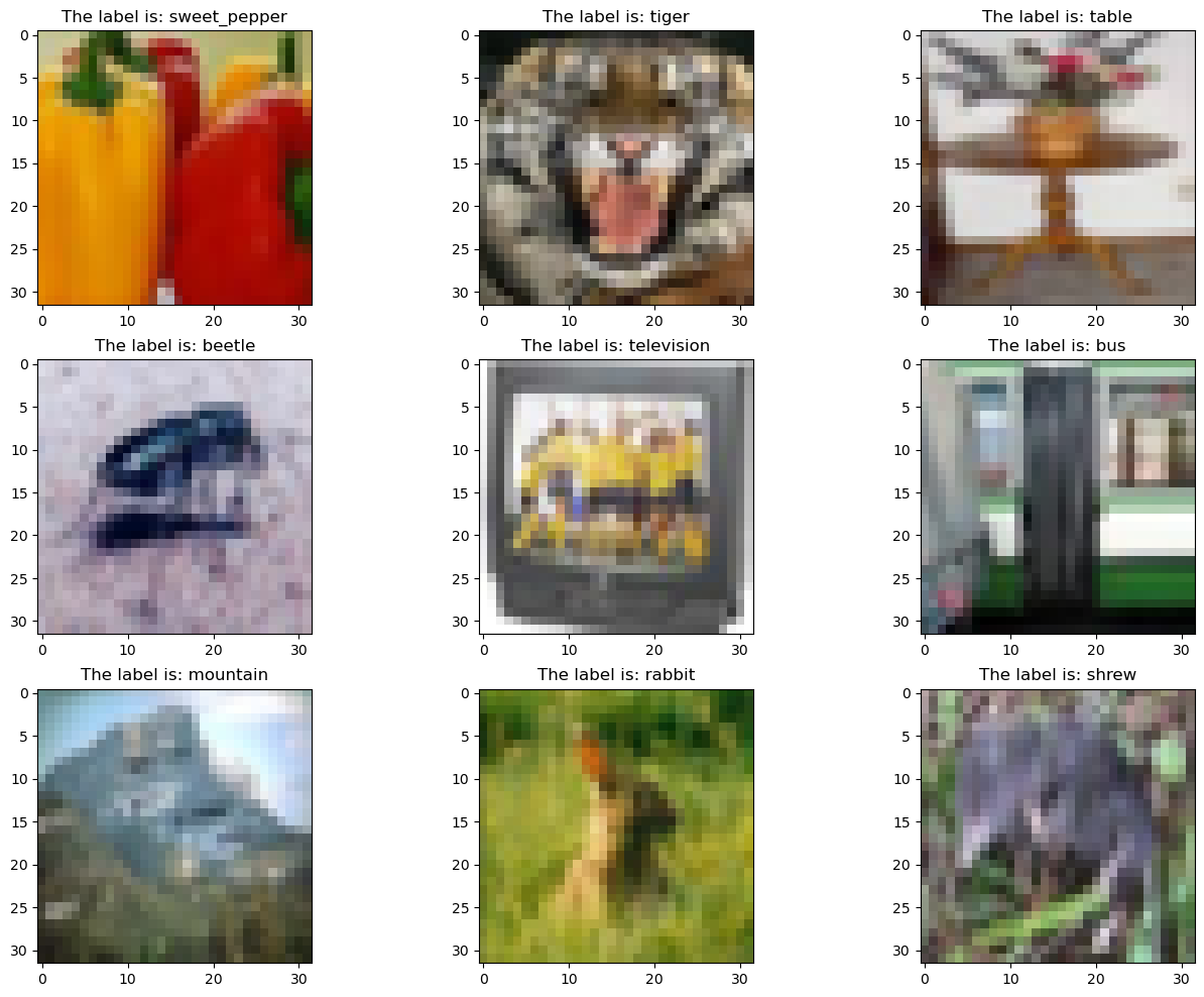
Plot nine random CIFAR100 images using matplotlib
1
2
3
4
5
6
7
|
random_idx = np.random.randint(1, len(train_split), size=9)
fig, axes = plt.subplots(3, 3, figsize=(16, 12))

for idx, ax in enumerate(axes.ravel()):
    randIndex = random_idx[idx]
    ax.set_title('The label is: ' + textLabel[train_split[randIndex][1]])
    ax.imshow(train_split[randIndex][0])
|
1
2
|
print(train_split)
print(test_split)
|
Dataset CIFAR100
    Number of datapoints: 50000
    Root location: ./cifar-100
    Split: Train
Dataset CIFAR100
    Number of datapoints: 10000
    Root location: ./cifar-100
    Split: Test
Split
We first do a 80/20 train test stratify split by label
1
|
labels = [train_split[i][1] for i in range(len(train_split))]
|
1
|
train_list, valid_list = train_test_split(train_split, test_size=0.2, shuffle=True, stratify=labels) #, stratify=[i[1] for i in train_split]
|
Here we are inspecting the distribution of the variables, the x axis is the class labels in numbers, the y axis the count for that class.
1
2
3
4
5
|
import plotly.express as px
x = [train_list[i][1] for i in range(len(train_list))]
fig = px.histogram(x)
fig.update_layout(title="Train list",bargap=0.2)
fig.show()
|
1
2
3
4
|
x = [valid_list[i][1] for i in range(len(valid_list))]
fig = px.histogram(title="Valid list", y=x)
fig.update_layout(bargap=0.2)
fig.show()
|
1
2
3
4
|
x = [test_split[i][1] for i in range(len(test_split))]
fig = px.histogram(x)
fig.update_layout(title="Test list",bargap=0.2)
fig.show()
|
1
2
3
|
print(f"Train Data: {len(train_list)}")
print(f"Validation Data: {len(valid_list)}")
print(f"Test Data: {len(test_split)}")
|
Train Data: 40000
Validation Data: 10000
Test Data: 10000
Datasets Loading and Argumentations
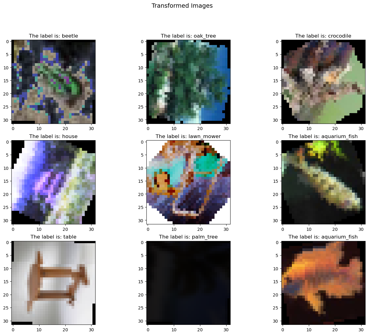
Here we define the data argumentations and create data loaders for each data split.
 1
 2
 3
 4
 5
 6
 7
 8
 9
10
11
12
13
14
15
16
17
18
19
20
21
22
23
|
from torchvision.transforms.autoaugment import AutoAugmentPolicy

all_transforms = transforms.Compose([
                    transforms.RandomHorizontalFlip(),
                    transforms.RandomVerticalFlip(),
                    transforms.RandomRotation(degrees=(0, 180)),
                    transforms.ColorJitter(brightness=0, contrast=0, saturation=0, hue=0),
                    transforms.AutoAugment(AutoAugmentPolicy.CIFAR10),
                    transforms.ToTensor(),
                    # transforms.RandomErasing(),
                ])

val_transforms = transforms.Compose(
    [
        transforms.ToTensor(),
    ]
)

test_transforms = transforms.Compose(
    [
        transforms.ToTensor(),
    ]
)
|
Here we are defining our own data class with transforms.
 1
 2
 3
 4
 5
 6
 7
 8
 9
10
11
12
13
14
15
16
|
class CIFAR100Dataset(Dataset):
    def __init__(self, rawData, transform=None):
        self.rawData = rawData
        self.transform = transform

    def __len__(self):
        self.dataSize = len(self.rawData)
        return self.dataSize

    def __getitem__(self, idx):
        rawData = self.rawData[idx]
        img = rawData[0]
        img_transformed = self.transform(img)
        label = rawData[1]

        return img_transformed, label
|
1
2
3
|
train_list_transformed = CIFAR100Dataset(train_list, transform=all_transforms)
valid_list_transformed= CIFAR100Dataset(valid_list, transform=val_transforms)
test_split_transformed= CIFAR100Dataset(test_split, transform=test_transforms)
|
 1
 2
 3
 4
 5
 6
 7
 8
 9
10
11
12
13
14
15
16
17
18
19
20
21
22
23
24
25
26
27
28
29
30
31
32
33
34
35
|
random_idx = np.random.randint(1, len(train_list_transformed), size=9)
fig, axes = plt.subplots(3, 3, figsize=(16, 12))
fig.suptitle("Transformed Images", fontsize=14)
for idx, ax in enumerate(axes.ravel()):
randIndex = random_idx[idx]
ax.set_title('The label is: ' + textLabel[train_list_transformed[randIndex][1]])
ax.imshow(transforms.ToPILImage()(train_list_transformed[randIndex][0]))
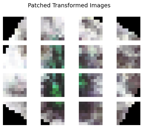
PATCH_SIZE = 8
PATCH_NUM = int(32 / PATCH_SIZE)
patches = train_list_transformed[random_idx[0]][0].unfold(1, PATCH_SIZE, PATCH_SIZE).unfold(2, PATCH_SIZE, PATCH_SIZE)
fig, ax = plt.subplots(PATCH_NUM, PATCH_NUM)
fig.suptitle("Patched Transformed Images", fontsize=14)
for i in range(PATCH_NUM):
for j in range(PATCH_NUM):
sub_img = patches[:, i, j]
ax[i][j].imshow(torchvision.transforms.functional.to_pil_image(sub_img))
ax[i][j].axis('off')
patches = patches.reshape(3, -1, PATCH_SIZE, PATCH_SIZE)
patches.transpose_(0, 1)
fig, ax = plt.subplots(1, PATCH_NUM*PATCH_NUM, figsize=(20, 20))
for i in range(PATCH_NUM**2):
ax[i].imshow(torchvision.transforms.functional.to_pil_image(patches[i]))
ax[i].axis('off')
fig, ax = plt.subplots(1, 4)
for i in range(4):
ax[i].imshow(torchvision.transforms.functional.to_pil_image(patches[i]))
ax[i].axis('off')
|


1
2
3
|
train_loader = torch.utils.data.DataLoader(train_list_transformed, batch_size=batchSize, shuffle=True)
valid_loader = torch.utils.data.DataLoader(valid_list_transformed, batch_size=batchSize, shuffle=True)
test_loader = torch.utils.data.DataLoader(test_split_transformed, batch_size=batchSize, shuffle=True)
|
1
|
print(len(train_list), len(train_loader))
|
40000 313
1
|
print(len(valid_list), len(valid_loader))
|
10000 79
Here we are inspecting the transformed data.
1
|
train_list_transformed[0]
|
(tensor([[[0.5176, 0.5882, 0.7255,  ..., 0.3451, 0.3882, 0.4431],
          [0.5255, 0.6431, 0.9882,  ..., 0.3059, 0.5255, 0.4706],
          [0.5255, 0.7255, 0.7333,  ..., 0.4000, 0.6000, 0.4353],
          ...,
          [0.9882, 0.8784, 0.6980,  ..., 0.1529, 0.1725, 0.2784],
          [0.9804, 0.8627, 0.6784,  ..., 0.2000, 0.2706, 0.4431],
          [0.9882, 0.8784, 0.7176,  ..., 0.2510, 0.4078, 0.5608]],

         [[0.4431, 0.5255, 0.6627,  ..., 0.3529, 0.4000, 0.4510],
          [0.4627, 0.5804, 0.6980,  ..., 0.3176, 0.5333, 0.4784],
          [0.4510, 0.6627, 0.6706,  ..., 0.4078, 0.6078, 0.4431],
          ...,
          [0.6980, 0.9333, 0.7451,  ..., 0.1804, 0.2000, 0.3059],
          [0.7176, 0.9176, 0.7333,  ..., 0.2235, 0.2980, 0.4706],
          [0.6980, 0.9333, 0.7725,  ..., 0.2784, 0.4431, 0.6000]],

         [[0.0745, 0.1255, 0.2902,  ..., 0.3255, 0.3922, 0.4667],
          [0.0863, 0.2000, 0.3412,  ..., 0.2784, 0.5804, 0.5059],
          [0.0863, 0.3137, 0.3020,  ..., 0.4157, 0.6824, 0.4549],
          ...,
          [0.3137, 0.4275, 1.0000,  ..., 0.2510, 0.2784, 0.4275],
          [0.3412, 0.4549, 0.9725,  ..., 0.3137, 0.4039, 0.6431],
          [0.3255, 0.4392, 0.6431,  ..., 0.3922, 0.5686, 0.7686]]]),
 67)
1
2
3
4
5
|
train_list_transformed[0][0].shape
ch, seqDim, _ = train_list_transformed[0][0].shape
print(ch, seqDim)
print(train_list_transformed[0][0].shape)
print(len(train_list_transformed))
|
3 32
torch.Size([3, 32, 32])
40000
Efficient Attention
We want to use patch size of 8x8 for our CIFAR100 image which has 32x32 dimension.
Note: large patch size would make the model fail to predict objects with complex features.
Here we are using Linformer from paper Linformer: Self-Attention with Linear Complexity by Sinong Wang et al. The implementation of this transformer is provided by lucidrains.
1
2
3
4
5
6
|
dim: the dimension of each head in multi-head attention
k: the k that the key/values are projected to along the sequence dimension
heads: number of heads
dropout: the dropout rate for the linear layers
depth: number of transformer block
seq_len: the length of the sequence (number of pixels + class label)
|
1
2
3
4
5
6
7
8
|
efficient_transformer = Linformer(
    dim=256,
    seq_len=64+1,  # 8x8 patches + 1 cls-token
    depth=4,
    heads=8,
    k=64,
    dropout = 0.1
)
|
Construct the transformer model using the transformer defined above. The implementation of the model is provided by lucidrains’s vit-pytorch.
1
2
3
4
5
|
dim: Last dimension of output tensor after linear transformation
patch_size: Number of patches
image_size: dimension of the input image
num_classes: classes to classify
channels: color channels
|
1
2
3
4
5
6
7
8
|
model = ViT(
    dim=256,
    image_size=32,      # 32 pixel by 32 pixel image
    patch_size=4,       # Total 4 patch 8x8 each
    num_classes=100,
    transformer=efficient_transformer,
    channels=3
).to(device)
|
We decided to use SGD for classification over all other optimizers for our task after a lot of research and experiment. Adam and RMSprop didn’t perform as well as SGD. A basic scheduler was added to prevent overshoot according to our past experiment where 30% valid accuracy seems to be a barrier. The scheduler was set to decay the learning rate every 10 epoch at 80 percent.
1
2
3
4
5
6
7
|
# loss function
criterion = nn.CrossEntropyLoss()
# optimizer
lr = 5e-3
optimizer = optim.SGD(model.parameters(), lr=lr, momentum=0.99) # weight_decay=0.01
# optimizer = optim.Adam(model.parameters(), lr=lr, weight_decay=5e-5) # weight_decay=0.01
scheduler = StepLR(optimizer, step_size=10, gamma=0.8)
|
1
2
|
records = []        # A variable to record data for each epoch so we can save the data in a csv later
# model = torch.load('./argumentModel', map_location=device)
|
1
2
|
# Waking from suspend cause the nvidia driver to fail sometimes, this command remove and add nvidia_uvm module to solve this problem
# !sudo modprobe -r nvidia_uvm && sudo modprobe nvidia_uvm
|
We are using a mixed precision training here to speed up the training process.
 1
 2
 3
 4
 5
 6
 7
 8
 9
10
11
12
13
14
15
16
17
18
19
20
21
22
23
24
25
26
27
28
29
30
31
32
33
34
35
36
37
38
39
40
41
42
43
44
45
46
|
scaler = torch.cuda.amp.GradScaler(enabled=True)
model.train()

for epoch in range(200):
    epoch_loss = 0
    epoch_accuracy = 0
    for data, label in tqdm(train_loader):
        data = data.to(device)
        label = label.to(device)

        with torch.autocast(device_type='cuda', dtype=torch.float16):
            output = model(data)
            assert output.dtype is torch.float16
            loss = criterion(output, label)
            assert loss.dtype is torch.float32

        scaler.scale(loss).backward()
        # loss.backward()

        scaler.step(optimizer)
        # scheduler.step()
        # optimizer.step()
        scaler.update()
        optimizer.zero_grad()

        acc = (output.argmax(dim=1) == label).float().mean()
        epoch_accuracy += acc / len(train_loader)
        epoch_loss += loss / len(train_loader)

    with torch.no_grad():
        epoch_val_accuracy = 0
        epoch_val_loss = 0
        for data, label in valid_loader:
            data = data.to(device)
            label = label.to(device)

            val_output = model(data)
            val_loss = criterion(val_output, label)

            acc = (val_output.argmax(dim=1) == label).float().mean()
            epoch_val_accuracy += acc / len(valid_loader)
            epoch_val_loss += val_loss / len(valid_loader)
    records.append([int(epoch+1), epoch_loss.detach().cpu().numpy(), epoch_accuracy.detach().cpu().numpy(), epoch_val_loss.detach().cpu().numpy(), epoch_val_accuracy.detach().cpu().numpy()])
    print(
        f"Epoch : {epoch+1} - loss : {epoch_loss:.4f} - acc: {epoch_accuracy:.4f} - val_loss : {epoch_val_loss:.4f} - val_acc: {epoch_val_accuracy:.4f}\n"
    )
|
1
2
|
pytorch_total_params = sum(p.numel() for p in model.parameters())
"Total Model parameters: " + str(pytorch_total_params)
|
'Total Model parameters: 3245508'
We save the training datas into a csv file.
1
2
3
4
5
6
7
8
9
|
# Remove epoch use index instead
def saveModel(modelName):
    torch.save(model, './' + modelName)
    df = pd.DataFrame(np.array(records), columns=['epoch', 'epoch_loss', 'epoch_accuracy', 'epoch_val_loss', 'epoch_val_accuracy'])
    with open('./' + modelName + '.csv', 'a') as file:
        df.to_csv('./' + modelName + '.csv', mode='a', index=False)
        file.close()
    return df
saveModel('argumentModel3m')
|
|
epoch |
epoch_loss |
epoch_accuracy |
epoch_val_loss |
epoch_val_accuracy |
| 0 |
1.0 |
4.733254 |
0.011282 |
4.483023 |
0.020965 |
| 1 |
2.0 |
4.468264 |
0.025909 |
4.345340 |
0.039953 |
| 2 |
3.0 |
4.409954 |
0.033072 |
4.277212 |
0.046183 |
| 3 |
4.0 |
4.363261 |
0.037640 |
4.194314 |
0.049150 |
| 4 |
5.0 |
4.269330 |
0.052741 |
4.093012 |
0.071104 |
| ... |
... |
... |
... |
... |
... |
| 367 |
168.0 |
0.801882 |
0.782972 |
3.416599 |
0.398141 |
| 368 |
169.0 |
0.807127 |
0.779703 |
3.434716 |
0.401800 |
| 369 |
170.0 |
0.790040 |
0.789462 |
3.495779 |
0.403085 |
| 370 |
171.0 |
0.802609 |
0.784545 |
3.469838 |
0.404371 |
| 371 |
172.0 |
0.815568 |
0.778655 |
3.411168 |
0.407437 |
372 rows × 5 columns
1
2
|
def getModelCSV(modelName):
    return pd.read_csv('./' + modelName + '.csv')
|
1
2
3
4
5
6
|
import hvplot.pandas
def getModelPlot(modelName):
    return getModelCSV(modelName).hvplot(title=f'{modelName}', xlabel='epoch', ylabel='%', use_index=True,
                                         y=['epoch_loss', 'epoch_accuracy', 'epoch_val_loss', 'epoch_val_accuracy'], kind='line')

getModelPlot('argumentModel3m')
|
Output Samples
 1
 2
 3
 4
 5
 6
 7
 8
 9
10
11
12
13
|
random_idx = np.random.randint(1, len(valid_list_transformed), size=9)
fig, axes = plt.subplots(3, 3, figsize=(16, 12))
model.eval()

for idx, ax in enumerate(axes.ravel()):
    randIndex = random_idx[idx]
    # input tensor must be [batch size, channels, h, w]
    predictLabel = model(valid_list_transformed[randIndex][0].unsqueeze(0).to(device)).argmax(dim=1)
    trueLabel = valid_list_transformed[randIndex][1]

    ax.set_title('Prediction: ' + textLabel[predictLabel] + '\n'
                 + 'True Label: ' + textLabel[trueLabel])
    ax.imshow(transforms.ToPILImage()(valid_list_transformed[randIndex][0]))
|

Future Works
The large patch size might caused be the cause for the model to fail on complex shapes, but the model was able to succuessfully capture common patterns in simple objects as shown above. We could improve the prediction on complex images by implementing a Compact Convolutional Transformers or use a Not All Images are Worth 16x16 Words: Dynamic Transformers for Efficient Image Recognition that dynamically reduce the patch size to better predict complex images.